next up previous
Next: Thermodynamic Forces & Kinetic Up: Time Dependent Fluctuations Previous: Time Dependent Fluctuations

Subsections


Relaxation & Time Correlation Function

Relaxation Time

Suppose we have a thermodynamic variable x with $\left\langle x\right\rangle=0$. What happens if at some moment $x=x_0\ne0$?

Thermodynamics Language:
We have a restricted ensemble: a set of systems with the given x.
Example:
I prepared a set of beakers at the temperature T0 and put it in the thermostat with the temperature T.
Kinetics and Equilibrium:
A beaker at the temperature T is not in the equilibrium with the environment--technically speaking, we cannot use thermodynamics!
A Trick:
we say that it is partially equilibrated--everything is equilibrated for this temperature.
General situation:
we have a slowly changing variable x, and say, that every other degree of freedom is fast.
Then we have a function $\left\langle x(t)\right\rangle$, such as  
 \begin{displaymath}
 \left\langle x(0)\right\rangle=x_0\end{displaymath} (1)

At $\left\langle x\right\rangle=0$ we have $d\left\langle x\right\rangle/dt=0$ (why?). For small deviations $d\left\langle x\right\rangle/dt$ is small. We can expand it in series in $\left\langle x\right\rangle$, and  
 \begin{displaymath}
 \frac{d\left\langle x\right\rangle}{dt} = -\lambda\left\langle x\right\rangle,\quad \lambda\gt\end{displaymath} (2)
Solution:  
 \begin{displaymath}
 \left\langle x(t)\right\rangle=x_0e^{-\lambda t}, \quad t\gt\end{displaymath} (3)
Small fluctuations decay exponentially with the relaxation time $\tau=1/\lambda$.

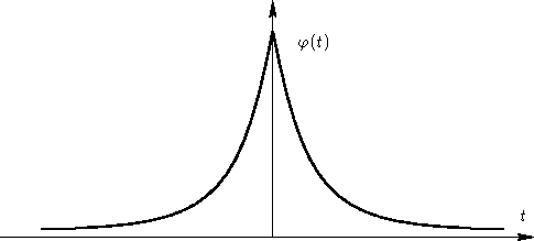
This formula is valid only for t>0: we can prepare an ensemble with given x0 and observe it, but cannot go backward! This is another manifestation of time irreversibility.

Time Correlation Function

For space-dependent problems we defined the correlation function $\left\langle x(\mathbf{0})x(\mathbf{r})\right\rangle$. For time-dependent case we define time correlation function $\varphi(t)=\left\langle x(0)x(t)\right\rangle$. We want to calculate $\varphi(t)$. This is the averaging over the ensemble of systems with arbitrary x(0). Note this difference with the previous case: there we had x(0) fixed, and used restricted ensembles. Now we return to the general case and consider equilibrium ensemble.

Translation along the time axis:

\begin{displaymath}
\left\langle x(t_1)x(t_2)\right\rangle=\left\langle x(0)x(t_2-t_1)\right\rangle=\varphi(t_2-t_1)\end{displaymath}

and therefore  
 \begin{displaymath}
 \varphi(-t)=\varphi(t)\end{displaymath} (4)

Double averaging method:

1.
Divide the ensemble into subensembles with given x(0)=xi. Each subensemble has many microscopic states with given macroscopic value x(0).
2.
Average x(0)x(t) in a subensemble:

\begin{displaymath}
\Phi(x_i,t) = \left\langle x_ix(t)\right\rangle_{\text{sub}}
 \end{displaymath}

3.
Average $\Phi(x_i,t)$ over all subensembles:

\begin{displaymath}
\varphi(t) = \left\langle \Phi(x_i,t)\right\rangle
 \end{displaymath}


\begin{figure}
\InputIfFileExists{ensembles.tex}{}{}\end{figure}

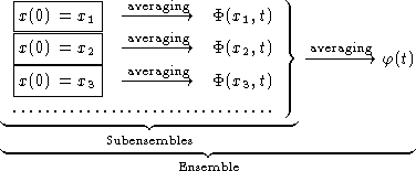
Since in a subensemble x(0) is given,

\begin{displaymath}
\Phi(x_0,t) =
 \left\langle x_0x(t)\right\rangle_{\text{sub}...
 ...left\langle x(t)\right\rangle_{\text{sub}}=x_0^2e^{-\lambda t} \end{displaymath}

Second averaging:

\begin{displaymath}
\left\langle x_0^2e^{-\lambda t}\right\rangle = \left\langle...
 ...right\rangle e^{-\lambda t} =
 \frac{kT}{\gamma}e^{-\lambda t} \end{displaymath}

with generalized susceptibility $\gamma$.

We obtained for the correlation function:

\begin{displaymath}
\varphi(t)=\frac{kT}{\gamma}e^{-\lambda t},\quad t\gt \end{displaymath}

From (4) we obtain for negative t that $\varphi(t)\sim
e^{\lambda t}$, or  
 \begin{displaymath}
 \varphi(t)=\frac{kT}{\gamma}e^{-\lambda \left\lvert t\right\rvert}\end{displaymath} (5)

\begin{figure}
 \psfrag{t}{$t$}
 \psfrag{f}{$\varphi(t)$}
 \includegraphics{phi}\end{figure}
This function has different derivatives at $t\pm0$: time irreversibility!

Multi-Variate Case

Kinetic Equations

We have several variables xi. Kinetic equations:
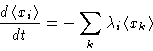
\begin{displaymath}
\frac{d\left\langle x_i\right\rangle}{dt}=-\sum_k \lambda_i \left\langle x_k\right\rangle\end{displaymath}

Now we have multi-variate correlation functions:

\begin{displaymath}
\varphi_{ij}(t) = \left\langle x_i(0)x_j(t)\right\rangle \end{displaymath}

Symmetry properties

1.
Translation of the time axis:

\begin{displaymath}
\left\langle x_i(t_1)x_j(t_2)\right\rangle=\left\langle x_i(0)x_j(t_2-t_1)\right\rangle=\varphi_{ij}(t_2-t_1)
 \end{displaymath}

We see:  
 \begin{displaymath}
 \varphi_{ij}(t)=\varphi_{ji}(-t)
 \end{displaymath} (6)
2.
Equations of motion are symmetric with respect to time inversion $t\to-t$:  
 \begin{displaymath}
 \varphi_{ij}(t)=\varphi_{ij}(-t)
 \end{displaymath} (7)
3.
From (6) and (7)  
 \begin{displaymath}
 \varphi_{ij}(t)=\varphi_{ji}(t)
 \end{displaymath} (8)

next up previous
Next: Thermodynamic Forces & Kinetic Up: Time Dependent Fluctuations Previous: Time Dependent Fluctuations

© 1997 Boris Veytsman and Michael Kotelyanskii
Tue Oct 28 22:13:33 EST 1997