


Next: Geometric Interpretation and Phase
Up: Phase Equilibria
Previous: Phase Equilibria
Subsections
- Homogeneous state:
- All part of my system are alike
- Inhomogeneous state:
- Some parts are different:
- Definition:
- Macroscopic states, coexisting at different
conditions, are called phases. Each phase exists in the
thermodynamic limit

- Question:
- Is microphase separation in co-polymers a true
phase equilibrium?

- Answer:
- No, we do not have separate independent macroscopic
phases! This is just one microscopically inhomogeneous
macroscopic phase.
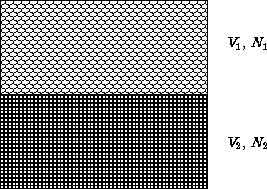
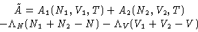
Suppose our system is at constant temperature. Total free energy is
|
A(N1,N2,V1,V2,T) = A1(N1,V1,T) + A2(N2,V2,T)
|
(1) |
with
| 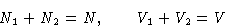 |
(2) |
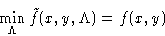
We want to minimize (1) under conditions (2).
We want to minimize f(x,y) under conditions g(x,y)=0. Construct a
new function
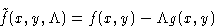
and minimize this as function of independent variables x, y,
 . Minimizing by we obtain g(x,y)=0, i.e.
- Example:
- I want to fence a rectangular lot of the given area
A. How can I save money on the fence?
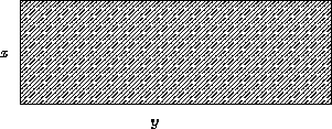
- Solution:
- For an
 lot the area is A=xy, the fence
is f=2x+2y long. We want to minimize
lot the area is A=xy, the fence
is f=2x+2y long. We want to minimize

We minimize:

and obtain

The result is  --I'd better make a square lot.
To minimize free energy (1) under conditions (2), we
minimize a new function
|  |
(3) |
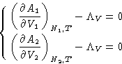
The derivatives here are just (minus) pressures! We obtained:
- 1.
- In equilibrium both phases have equal pressures (mechanic
equilibrium) P1=P2=P
- 2.
- Lagrange multiplier
 is minus pressure of the system:

- 1.
- Both phases have equal chemical potentials

- 2.
- Lagrange multiplier
 is the chemical potential of the
system:
is the chemical potential of the
system: 
In coexisting phase P, T,  are equal (as well as other
thermodynamic fields).
are equal (as well as other
thermodynamic fields).
Let's forget about phase 2. The condition for N1 for phase 1
can be obtained from minimization a function
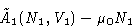
with external pressure and chemical potential P0 and  .In equilibrium
  is
is  -potential (we already derived
this in previous
lectures
).
-potential (we already derived
this in previous
lectures
).
The extremum should be a minimum  second derivatives are
positive!
second derivatives are
positive!
Suppose we have an extensive variable xi. It has
conjugated field
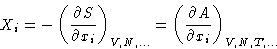
In equilibrium Xi is constant in all phases, and the matrix
 with
with
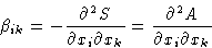
is positive (in equilibrium S has maximum, and A minimum!).
We can obtain this by minimizing
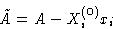
with external value Xi(0)
Next: Geometric Interpretation and Phase
Up: Phase Equilibria
Previous: Phase Equilibria
© 1997
Boris Veytsman
and Michael Kotelyanskii
Thu Oct 2 21:02:12 EDT 1997